A test of normality. We derive the W statistic from generalized least squares on the order statistics, and cover its location–scale invariance, its independence of (X̄, S²), its exact distribution for n = 3, Royston’s approximation, and power.
Published
September 30, 2026
WarningDraft — not yet peer-reviewed
The proofs in this article are a draft and have not yet been reviewed or edited.
Scope
For a single sample \(X_1,\dots,X_n\) we consider the following test.
Null hypothesis
Alternative
\(X_1,\dots,X_n\iid N(\mu,\sigma^2)\) for some \(\mu\in\R\), \(\sigma>0\)
Not normally distributed
The mean and variance are not specified (any normal distribution is allowed). To test fit to a normal distribution with a specified mean and variance, the Kolmogorov–Smirnov test is more direct.
Using this tool
Required data
Data
Form
Notes
Sample \(x\)
Array of numbers (3 to 5,000 values)
Order does not matter (sorted internally)
Assumptions
Independent and identically distributed: the observations are independent and follow the same distribution. Serial autocorrelation, or a mixture of groups with different means, makes the data more likely to be judged non-normal.
Continuous distribution: many rounded values or ties (equal values) make rejection more likely even for data from a normal distribution (see Caveats).
Size: 3 to 5,000 values. The p-value approximation (Royston 1995) has been validated in this range. If all values are equal, the statistic cannot be computed.
Output
Value
Meaning
statistic
\(W\) (\(0<W\le1\); the closer to 1, the more consistent with normality)
pvalue
p-value (smaller for smaller \(W\))
n, mean, sd
Sample size, mean and standard deviation (divisor \(n-1\))
null_hypothesis
The null hypothesis
What we show
\(W\) measures how close the normal Q-Q plot is to a straight line, using the idea of generalized least squares on the order statistics. Starting from the definition, we show the following.
\(W\) is invariant under changes of location and scale, and equals the squared correlation coefficient between the coefficient vector and the order statistics (hence \(W\le1\)).
Under the null hypothesis, \(W\) is independent of \((\bar X,S^2)\). The distribution of \(W\) does not depend on \(\mu,\sigma\).
For \(n=3\) the distribution of \(W\) can be found exactly: \(P(W\le w)=\frac6\pi\big(\arcsin\sqrt w-\frac\pi3\big)\).
For \(n\ge4\) the distribution has no closed form. We present the Royston (1995) approximation used by the API and on this site, and check by simulation that the significance level is maintained and how much power the test has.
Definition of W
A linear model for the order statistics
Let \(X_i=\mu+\sigma Z_i\) with \(Z_i\iid N(0,1)\), and write the sorted values as \(X_{(1)}\le\dots\le X_{(n)}\) and \(Z_{(1)}\le\dots\le Z_{(n)}\). Since \(\sigma>0\), sorting commutes with the affine map, so \(X_{(i)}=\mu+\sigma Z_{(i)}\). Denote the means and covariances of the standard normal order statistics by \[
m_i=\E Z_{(i)},\qquad V_{ij}=\Cov\big(Z_{(i)},Z_{(j)}\big).
\] Then \(\boldsymbol x=(X_{(1)},\dots,X_{(n)})^\top\) follows the linear model (with correlated errors) \[
\boldsymbol x=\mu\boldsymbol 1+\sigma\boldsymbol m+\boldsymbol\varepsilon,\qquad \E\boldsymbol\varepsilon=\boldsymbol 0,\quad \Var\boldsymbol\varepsilon=\sigma^2V .
\] The points \((m_i,X_{(i)})\) form the normal Q-Q plot, and the model says that “the Q-Q plot scatters around a straight line with slope \(\sigma\).”
Symmetry
The variables \(-Z_1,\dots,-Z_n\) are also independent \(N(0,1)\), and the \(i\)-th smallest of them is \(-Z_{(n+1-i)}\). Hence \[
\big(Z_{(1)},\dots,Z_{(n)}\big)\overset{d}{=}\big(-Z_{(n)},\dots,-Z_{(1)}\big).
\] Letting \(J\) be the order-reversing matrix (\(J_{ij}=1\iff i+j=n+1\)), it follows that \(J\boldsymbol m=-\boldsymbol m\) and \(JVJ=V\). In particular, \(\boldsymbol 1^\top\boldsymbol m=\boldsymbol 1^\top J\boldsymbol m=-\boldsymbol 1^\top\boldsymbol m\), so \(\boldsymbol 1^\top\boldsymbol m=0\).
The best linear unbiased estimator of σ, and W
Since \(\boldsymbol 1^\top V^{-1}\boldsymbol m=0\) (by the lemma below), the best linear unbiased estimator of \(\sigma\) obtained by generalized least squares (Lloyd 1952) is \[
\hat\sigma=\frac{\boldsymbol m^\top V^{-1}\boldsymbol x}{\boldsymbol m^\top V^{-1}\boldsymbol m}.
\] Using the normalized coefficients \[
\boldsymbol a=\frac{V^{-1}\boldsymbol m}{\big\|V^{-1}\boldsymbol m\big\|}\qquad(\|\boldsymbol a\|=1),
\] Shapiro and Wilk (1965) defined \[
W=\frac{\big(\sum_{i=1}^n a_iX_{(i)}\big)^2}{\sum_{i=1}^n(X_i-\bar X)^2}.
\] The numerator is a constant multiple of \(\hat\sigma^2\) and the denominator is \((n-1)S^2\); under normality, both estimate \(\sigma^2\). If the distribution is not normal, the Q-Q plot bends, and the numerator (the scale obtained from the slope of the line) becomes smaller than the denominator.
Lemma.\(J\boldsymbol a=-\boldsymbol a\). In particular, \(a_i=-a_{n+1-i}\) and \(\sum_ia_i=0\).
Proof. From \(J^2=I\) and \(JVJ=V\) we get \(JV^{-1}J=V^{-1}\), i.e. \(JV^{-1}=V^{-1}J\). Hence \(JV^{-1}\boldsymbol m=V^{-1}J\boldsymbol m=-V^{-1}\boldsymbol m\). Since \(J\boldsymbol1=\boldsymbol1\), we have \(\boldsymbol 1^\top\boldsymbol a=\boldsymbol 1^\top J\boldsymbol a=-\boldsymbol 1^\top\boldsymbol a\), so the sum is 0. \(\square\)
Theorem 1 (Invariance and representation as a correlation)
For \(c\in\R\) and \(b>0\), replacing each \(X_i\) by \(c+bX_i\) leaves \(W\) unchanged.
\(W\) is the squared correlation coefficient between \((a_1,\dots,a_n)\) and \((X_{(1)},\dots,X_{(n)})\). Hence \(0\le W\le1\).
Proof. 1. Since \(b>0\), the order statistics become \(c+bX_{(i)}\). By the lemma, \(\sum_ia_i(c+bX_{(i)})=b\sum_ia_iX_{(i)}\), and the denominator is multiplied by \(b^2\), so the ratio is unchanged.
Since \(\sum_ia_i=0\), we have \(\sum_ia_iX_{(i)}=\sum_ia_i(X_{(i)}-\bar X)\); moreover \(\sum_i(X_i-\bar X)^2=\sum_i(X_{(i)}-\bar X)^2\). Using \(\sum_ia_i^2=1\) and \(\bar a=0\), \[
W=\frac{\big(\sum_i(a_i-\bar a)(X_{(i)}-\bar X)\big)^2}{\sum_i(a_i-\bar a)^2\,\sum_i(X_{(i)}-\bar X)^2}=\Corr\big(\boldsymbol a,\boldsymbol x\big)^2 .
\] By the Cauchy–Schwarz inequality, \(W\le1\). \(\square\)
Equality \(W=1\) holds only when \(X_{(i)}\) is an affine function of \(a_i\). A lower bound is \(W\ge na_1^2/(n-1)\) (Shapiro and Wilk 1965, Lemma 1).
Theorem 2 (Independence of \((\bar X,S^2)\))
Under the null hypothesis, the distribution of \(W\) does not depend on \((\mu,\sigma)\), and \(W\) is independent of \((\bar X,S^2)\).
Proof. Taking \(c=-\mu/\sigma\) and \(b=1/\sigma\) in part 1 of Theorem 1 gives \(W(X_1,\dots,X_n)=W(Z_1,\dots,Z_n)\), whose distribution involves no parameters (\(W\) is an ancillary statistic). On the other hand, \((\bar X,S^2)\) is a complete sufficient statistic for the normal family \(\{N(\mu,\sigma^2)^{\otimes n}\}\) (a two-parameter exponential family whose natural parameter space contains an open subset of \(\R^2\)). By Basu’s theorem (Theorem C in the t-test article (Japanese)), an ancillary statistic is independent of a complete sufficient statistic. \(\square\)
Corollary. In \(\big(\sum_ia_iX_{(i)}\big)^2=W\cdot(n-1)S^2\) the two factors on the right are independent, so for \(k=1,2,\dots\)\[
\E W^k=\frac{\E\big(\sum_ia_iX_{(i)}\big)^{2k}}{\E\big((n-1)S^2\big)^k} .
\] For \(k=1\), using \(\E(\boldsymbol a^\top\boldsymbol x)^2=\sigma^2\big(\boldsymbol a^\top V\boldsymbol a+(\boldsymbol a^\top\boldsymbol m)^2\big)\) (since \(\boldsymbol a^\top\boldsymbol 1=0\)) and \(\E(n-1)S^2=(n-1)\sigma^2\), \[
\E W=\frac{\boldsymbol a^\top V\boldsymbol a+(\boldsymbol a^\top\boldsymbol m)^2}{n-1} .
\] It is independence that makes the expectation of the ratio equal to the ratio of expectations; Shapiro and Wilk (1965) obtained the low-order moments of \(W\) in this way.
Theorem 3 (Exact distribution for \(n=3\))
For \(n=3\), \(\boldsymbol a=(-1/\sqrt2,\,0,\,1/\sqrt2)\), and under the null hypothesis \(W\) takes values in \([3/4,1]\) with \[
P(W\le w)=\frac6\pi\Big(\arcsin\sqrt w-\frac\pi3\Big),\qquad \frac34\le w\le1 .
\]
Proof. By the lemma, \(a_2=0\) and \(a_3=-a_1\); together with \(\|\boldsymbol a\|=1\) this gives the form above, and \(W=(X_{(3)}-X_{(1)})^2/\big(2\sum_i(X_i-\bar X)^2\big)\). By Theorem 2 we may take \(\mu=0,\sigma=1\).
The residual vector \(\boldsymbol e=(X_i-\bar X)_i\) is the orthogonal projection of \(\boldsymbol Z\) onto the plane \(P\) orthogonal to \(\boldsymbol 1\). Since the distribution of a standard normal vector is rotation invariant, \(\boldsymbol e/\|\boldsymbol e\|\) is uniformly distributed on the unit circle of \(P\). The unit circle of \(P\) can be parametrized as \[
\boldsymbol e/\|\boldsymbol e\|=\sqrt{\tfrac23}\,\big(\cos\theta,\ \cos(\theta-\tfrac{2\pi}3),\ \cos(\theta+\tfrac{2\pi}3)\big),\qquad \theta\in[0,2\pi)
\] (the three cosines sum to 0 and their squares sum to \(3/2\)), so \(\theta\) is uniformly distributed on \([0,2\pi)\).
\(W\) is unchanged by permuting the components of \(\boldsymbol e\), and permutations of the components correspond to \(\theta\mapsto\theta\pm\frac{2\pi}3\) and \(\theta\mapsto-\theta\). These maps carry the six intervals of length \(\pi/3\) partitioning \([0,2\pi)\) onto one another, so we may assume \(\theta\) is uniform on \([0,\pi/3]\). On this interval the largest component is \(\cos\theta\) and the smallest is \(\cos(\theta+\frac{2\pi}3)\), and \[
\cos\theta-\cos\big(\theta+\tfrac{2\pi}3\big)=2\sin\big(\theta+\tfrac\pi3\big)\sin\tfrac\pi3=\sqrt3\,\sin\big(\theta+\tfrac\pi3\big),
\qquad
W=\frac{\tfrac23\cdot3\sin^2(\theta+\frac\pi3)}{2}=\sin^2\varphi,
\] where \(\varphi=\theta+\frac\pi3\) is uniformly distributed on \([\frac\pi3,\frac{2\pi}3]\). Since \(\sin^2\) is symmetric about \(\varphi=\frac\pi2\), we may take \(\varphi\) uniform on \([\frac\pi3,\frac\pi2]\), where \(\sin\) is increasing. Therefore \[
P(W\le w)=P\big(\varphi\le\arcsin\sqrt w\big)=\frac{\arcsin\sqrt w-\pi/3}{\pi/2-\pi/3}=\frac6\pi\Big(\arcsin\sqrt w-\frac\pi3\Big).\qquad\square
\]
Smaller \(W\) means further from normality, so the p-value is \(P(W\le w_{\text{obs}})\). For \(n=3\) the API also computes the p-value from this formula.
Computing the coefficients and p-value (Royston’s approximation)
For \(n\ge4\), computing \(\boldsymbol m\) and \(V\) exactly is difficult, and Shapiro and Wilk (1965) tabulated the coefficients and quantiles for \(n\le50\). The API uses Royston’s (1992, 1995) approximation (AS R94), the same as R’s shapiro.test and scipy’s shapiro.
Coefficients. Replace \(m_i\) by Blom’s approximation \(\tilde m_i=\Phi^{-1}\big((i-\frac38)/(n+\frac14)\big)\) and set \(\boldsymbol a\approx\tilde{\boldsymbol m}/\|\tilde{\boldsymbol m}\|\) (this drops \(V^{-1}\), which is accurate enough for the coefficients near the middle). Only the extreme coefficients, where the error is large, are corrected by a fifth-degree polynomial in \(u=1/\sqrt n\): \[
a_n=\tilde c_n+0.221157u-0.147981u^2-2.071190u^3+4.434685u^4-2.706056u^5,
\] and for \(n>5\), \(a_{n-1}\) is corrected in the same way (\(\tilde c_i=\tilde m_i/\|\tilde{\boldsymbol m}\|\)). The remaining coefficients are rescaled so that \(\|\boldsymbol a\|=1\), and \(a_i=-a_{n+1-i}\) as in the lemma. For \(\Phi^{-1}\) we use Wichura’s (1988) AS241 (relative error about \(10^{-16}\)).
p-value. A transform of \(1-W\) is approximated by a normal distribution.
Here \(\ell=\log n\), and the p-value is \(P\big(N(\mu_n,\sigma_n^2)>y\big)\). In the extreme case \(\log(1-W)\ge\gamma\) with \(n\le11\), which lies outside the range of the approximation, the p-value is set to \(10^{-99}\), as in R and scipy. With \(s_a=\sum_i(a_i-\bar a)^2\), \(s_x=\sum_i(X_{(i)}-\bar X)^2\) and \(s_{ax}=\sum_i(a_i-\bar a)(X_{(i)}-\bar X)\) (Theorem 1, part 2), \(1-W\) is computed directly as \(\big(\sqrt{s_as_x}-s_{ax}\big)\big(\sqrt{s_as_x}+s_{ax}\big)/(s_as_x)\) to avoid cancellation when \(W\approx1\).
We have checked that the API’s results agree with scipy to within a relative error of \(10^{-9}\) on 2003 cases (\(n=3\) to \(5000\); normal, t, uniform, exponential and lognormal data, data with many ties, and data with a large mean and small variance).
Is the significance level maintained?
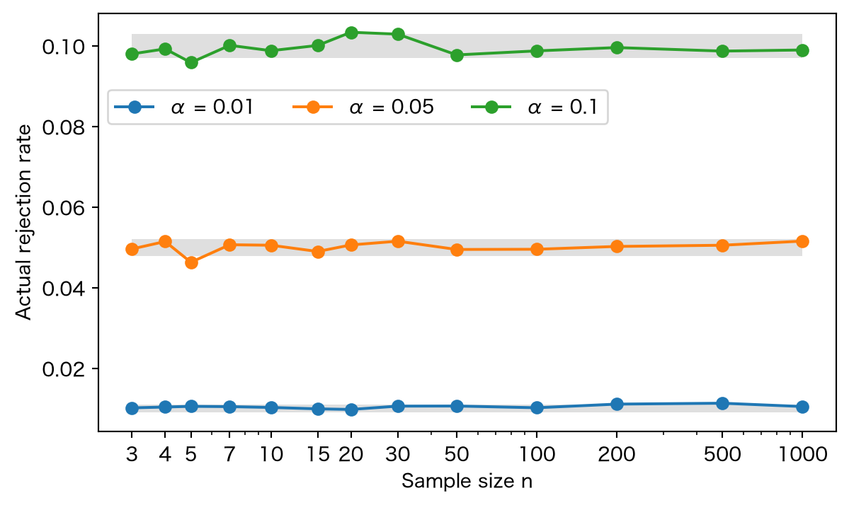
If the approximation works, the p-value is uniformly distributed under the null hypothesis, and the rejection rate equals the significance level.
Code
import numpy as npimport matplotlib.pyplot as pltfrom scipy import statsplt.rcParams["font.family"] = ["Hiragino Sans", "sans-serif"]rng = np.random.default_rng(0)reps =40000ns = [3, 4, 5, 7, 10, 15, 20, 30, 50, 100, 200, 500, 1000]alphas = [0.01, 0.05, 0.10]rate = {a: [] for a in alphas}for n in ns: x = rng.normal(size=(reps, n)) p = np.array([stats.shapiro(r).pvalue for r in x])for a in alphas: rate[a].append((p < a).mean())fig, ax = plt.subplots()for a in alphas: half =1.96* np.sqrt(a * (1- a) / reps) ax.fill_between(ns, a - half, a + half, color="gray", alpha=0.25, lw=0) ax.plot(ns, rate[a], "o-", label=f"α = {a}")ax.set_xscale("log")ax.set_xlabel("Sample size n")ax.set_xticks(ns, [str(n) for n in ns])ax.set_ylabel("Actual rejection rate")ax.legend(loc="upper left", bbox_to_anchor=(0, 0.84), ncols=3)plt.show()
Figure 1: Proportion of normal samples whose p-value falls below the significance level (40,000 replications for each n). The gray bands are the binomial 95% ranges.
For \(n=3\) the test is exact, and for \(n\ge4\) the rejection rate is also close to α at every significance level.
Power
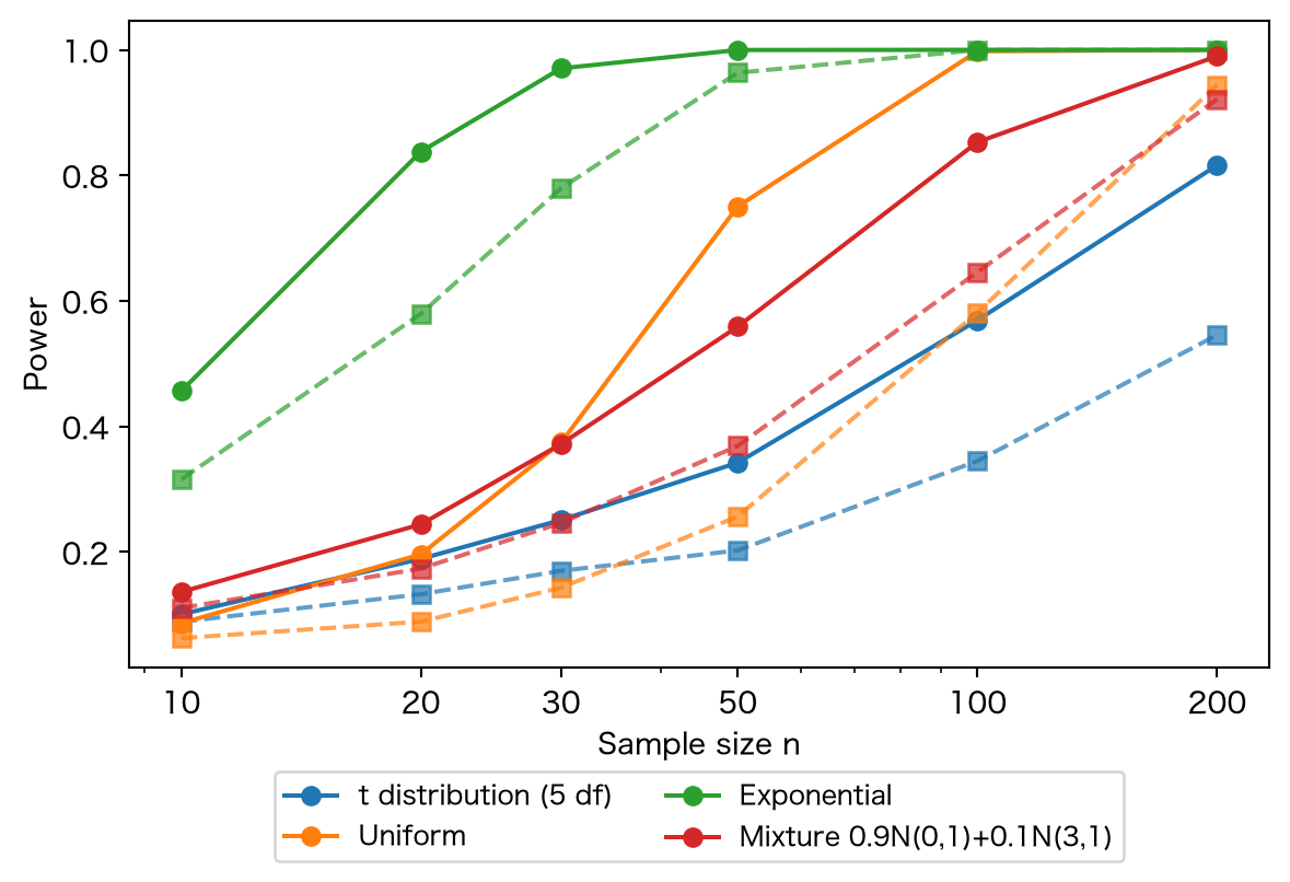
We compare how well the test detects non-normal samples with the Lilliefors test (the Kolmogorov–Smirnov distance to the fitted normal distribution), which likewise leaves the mean and variance unspecified.
Code
from statsmodels.stats.diagnostic import lillieforsalts = {"t distribution (5 df)": lambda size: rng.standard_t(5, size=size),"Uniform": lambda size: rng.uniform(size=size),"Exponential": lambda size: rng.exponential(size=size),"Mixture 0.9N(0,1)+0.1N(3,1)": lambda size: rng.normal(size=size) +3* (rng.uniform(size=size) <0.1),}ns = [10, 20, 30, 50, 100, 200]reps =4000fig, ax = plt.subplots()for name, gen in alts.items(): sw, lf = [], []for n in ns: x = gen((reps, n)) sw.append(np.mean([stats.shapiro(r).pvalue <0.05for r in x])) lf.append(np.mean([lilliefors(r, pvalmethod="table")[1] <0.05for r in x])) line, = ax.plot(ns, sw, "o-", label=name) ax.plot(ns, lf, "s--", color=line.get_color(), alpha=0.7)ax.set_xscale("log")ax.set_xticks(ns, [str(n) for n in ns])ax.set_xlabel("Sample size n")ax.set_ylabel("Power")ax.legend(fontsize=9, loc="upper center", bbox_to_anchor=(0.5, -0.14), ncols=2)plt.show()
Figure 2: Power at α = 0.05 (4,000 replications per point). Solid lines: Shapiro–Wilk; dashed lines: Lilliefors test.
Shapiro–Wilk has higher power against every alternative. Departures that show up in the tails rather than the center of the distribution, such as heavy tails (t distribution) or short tails (uniform), affect \(W\) strongly through the slope at the ends of the Q-Q plot. On the other hand, at \(n=20\) the test detects the t distribution (5 df) or the uniform distribution only about 20% of the time. A non-significant result is not evidence of normality.
Caveats
Large samples. When \(n\) is in the thousands, even small departures of no practical consequence give p-values near 0. To check the assumptions of a method that is robust by the central limit theorem, such as the t-test, look at the shape of the Q-Q plot rather than the p-value.
Ties and rounding. When values are rounded to a small number of distinct levels, the Q-Q plot becomes a staircase and \(W\) decreases. Even data from a normal distribution are more likely to be rejected if the measurement unit is coarse relative to the standard deviation.
Sequential testing. Choosing the next test based on the result, e.g. “use a t-test if the normality test is not significant, and a rank test if it is,” makes the overall type I error rate differ from the nominal α.
Use on residuals. Regression residuals are neither independent nor identically distributed, so the null distribution does not hold exactly. Use the result as a rough guide.
Try it
The same computation is available from the noisymoon API at POST /v1/tests/shapiro. \(W\) and the p-value agree with R’s shapiro.test and scipy’s shapiro.