Comparing location without distributional assumptions. The null distribution of ranks, the relation between U and the rank sum, means, variances and recursions for the exact distributions, tie corrections, power compared with the t-test, and the pitfall of unequal variances.
Published
September 30, 2026
WarningDraft — not yet peer-reviewed
The proofs in this article are a draft and have not yet been reviewed or edited.
Scope
We treat three tests that use only the ranks of the observations, not their values. Since they do not assume normality, they are robust to outliers and skewed distributions.
Test
Data
Null hypothesis
Corresponding t-test / ANOVA
Mann–Whitney U test (Wilcoxon rank-sum test)
Two independent samples \(x, y\)
\(x\) and \(y\) follow the same distribution
Two-sample t-test
Wilcoxon signed-rank test
One sample, or the differences \(d=x-y\) of paired samples
The distribution of \(d\) is symmetric about 0
One-sample / paired t-test
Kruskal–Wallis test
\(k\) independent groups
All groups follow the same distribution
One-way analysis of variance
Using this tool
Required data
Data
Form
Notes
Mann–Whitney: x, y
Arrays of numbers (1 to 100,000 values each)
Lengths may differ
Wilcoxon: x (and y)
Array of numbers
If y is given, the differences x − y are tested (same length)
Kruskal–Wallis: groups
Array of arrays of numbers (2 to 100 groups)
Groups can be named with labels
alternative
two-sided / greater / less
Mann–Whitney and Wilcoxon. greater means “\(x\) tends to be larger”
method
auto / exact / asymptotic
Exact distribution or normal approximation. auto chooses by the same rule as scipy (see below)
Independence: the observations are independent (for paired Wilcoxon, the pairs are independent).
A continuous distribution is ideal. Ties can be handled by a corrected approximation, but the exact distributions are those without ties.
The null hypothesis of Mann–Whitney and Kruskal–Wallis is “the distributions are the same”, not “the medians are the same”. When comparing groups with different variances or shapes, the significance level is not maintained (see below).
The null hypothesis of Wilcoxon is “symmetric about 0”. It cannot be used to test the median of a skewed distribution (use the sign test).
Output
Value
Meaning
statistic, pvalue, method
The statistic (\(U_1\) for Mann–Whitney; \(\min(R_+,R_-)\) two-sided and \(R_+\) one-sided for Wilcoxon; \(H\) for Kruskal–Wallis), the p-value, and the method used
z
Standardized statistic of the normal approximation (with asymptotic)
prob_superiority, rank_biserial
Mann–Whitney: \(\hat P(X>Y)+\frac12\hat P(X=Y)=U_1/(mn)\) and the rank-biserial correlation \(2U_1/(mn)-1\)
r_plus, r_minus, rank_biserial
Wilcoxon: rank sums of the positive and negative differences, and \((R_+-R_-)/(R_++R_-)\)
hodges_lehmann
Location estimate: the median of \(x_i-y_j\) for Mann–Whitney; the median of the Walsh averages \((d_i+d_j)/2\) (\(i\le j\)) for Wilcoxon
df, epsilon_squared, groups
Kruskal–Wallis: degrees of freedom \(k-1\), effect size \(H/(N-1)\), and for each group its size, mean rank and median
What we show
Under the null hypothesis the distribution of the ranks does not depend on the underlying distribution (the reason these are distribution-free tests).
The relation between the Mann–Whitney \(U\) and the rank sum, the mean and variance of \(U\) (including the tie correction), and a recursion for its exact distribution.
The Wilcoxon \(R_+\) is a weighted sum of independent Bernoulli variables; its mean, variance and exact distribution.
Two expressions for the Kruskal–Wallis \(H\), and the fact that for two groups \(H\) equals the square \(z^2\) of the Mann–Whitney normal approximation.
For asymptotic normality (and the asymptotic \(\chi^2\) distribution of \(H\)) we cite Lehmann (2006). Finally, we compare power with the t-test by simulation, and show an example in which the significance level breaks down when the variances differ.
Null distribution of the ranks
Let \(Z_1,\dots,Z_N\) be an independent sample from a continuous distribution, and let \(R_i\) be the rank of \(Z_i\) (its position counting from the smallest). Since the distribution is continuous, equal values occur with probability 0, and \((R_1,\dots,R_N)\) is a permutation of \(\{1,\dots,N\}\).
Lemma 1.\((R_1,\dots,R_N)\) is uniformly distributed over the \(N!\) permutations.
Proof. Since \(Z_1,\dots,Z_N\) are i.i.d., for every permutation \(\pi\) the vector \((Z_{\pi(1)},\dots,Z_{\pi(N)})\) has the same distribution as \((Z_1,\dots,Z_N)\) (exchangeability). For a permutation \(r\), \(P(R=r)=P(Z_{r^{-1}(1)}<\dots<Z_{r^{-1}(N)})\), which by exchangeability does not depend on \(r\). The \(N!\) probabilities sum to 1, so each equals \(1/N!\). \(\square\)
Corollary. Pool two samples \(X_1,\dots,X_m\iid F\) and \(Y_1,\dots,Y_n\iid G\) and rank them jointly. Under \(F=G\), the set of ranks of the \(X\)’s, \(\{R_1,\dots,R_m\}\), is uniformly distributed over the \(m\)-element subsets of \(\{1,\dots,N\}\) (\(N=m+n\)). The null distribution of any statistic that is a function of the ranks does not depend on \(F\) and is determined by \(m, n\) alone.
Mann–Whitney U test
U and the rank sum
Define \[
U_1=\#\{(i,j): X_i>Y_j\}\ \big(+\tfrac12\#\{(i,j): X_i=Y_j\}\big),\qquad W=\sum_{i=1}^m R_i
\] (\(W\) is the Wilcoxon rank sum).
Theorem 1.\(U_1=W-\dfrac{m(m+1)}{2}\).
Proof. When there are no ties, write the ranks of the \(X\)’s in increasing order as \(R_{(1)}<\dots<R_{(m)}\). There are \(R_{(i)}-1\) observations smaller than the \(i\)-th smallest \(X\); of these, \(i-1\) are \(X\)’s, so \(R_{(i)}-i\) are \(Y\)’s. Summing over \(i\) gives \(U_1=\sum_i(R_{(i)}-i)=W-m(m+1)/2\). When there are ties, using midranks counts each pair of an \(X\) and a \(Y\) with equal values as \(\frac12\), and the same formula holds. \(\square\)
\(U_2=mn-U_1\) is the same quantity with \(y\) as the reference, and \(U_1/(mn)\) is an unbiased estimator of \(\theta=P(X>Y)+\frac12P(X=Y)\) (prob_superiority). Under the null hypothesis \(F=G\), \(\theta=\frac12\).
Mean and variance
Theorem 2. Under \(F=G\) (continuous), \(\E U_1=\dfrac{mn}{2}\) and \(\Var U_1=\dfrac{mn(N+1)}{12}\).
Proof. By Lemma 1 each \(R_i\) is uniformly distributed on \(\{1,\dots,N\}\), so \(\E R_i=\frac{N+1}2\) and \(\Var R_i=\frac{N^2-1}{12}\). Since \(\sum_{i=1}^NR_i=N(N+1)/2\) is constant, \(0=\Var\sum_iR_i=N\Var R_1+N(N-1)\Cov(R_1,R_2)\), hence \(\Cov(R_i,R_j)=-\frac{N+1}{12}\) (\(i\ne j\)). \[
\Var W=m\frac{N^2-1}{12}-m(m-1)\frac{N+1}{12}=\frac{m(N+1)(N-m)}{12}=\frac{mn(N+1)}{12},
\] and \(\E W=m(N+1)/2\). The mean and variance of \(U_1\) follow from Theorem 1. \(\square\)
Tie correction. When tied observations receive midranks, the ranks are a permutation not of \(\{1,\dots,N\}\) but of the multiset of midranks \(a_1,\dots,a_N\) (the argument of Lemma 1 goes through unchanged if permutations of tied observations are not distinguished). Replacing a tie group of size \(t\) with ranks \(r,\dots,r+t-1\) by their mean reduces the sum of squared deviations by \(\sum_{s=0}^{t-1}(s-\frac{t-1}2)^2=\frac{t^3-t}{12}\). Therefore \(\sum_k(a_k-\bar a)^2=\frac{N^3-N-\sum(t^3-t)}{12}\). Since \(W\) is the sum of a sample of size \(m\) drawn without replacement from the population \(a\), the finite population correction gives \[
\Var U_1=\frac{mn}{N(N-1)}\sum_k(a_k-\bar a)^2=\frac{mn}{12}\Big((N+1)-\frac{\sum(t^3-t)}{N(N-1)}\Big).
\] The API’s normal approximation uses this variance, with \(z=(U_1-mn/2\mp\frac12)/\sqrt{\Var U_1}\) (the \(\mp\frac12\) is the continuity correction, applied in the direction that increases the p-value).
Proof. By exchangeability, the largest of the \(N\) observations is an \(X\) with probability \(m/N\). In that case this \(X\) exceeds every \(Y\) and contributes \(n\) to \(U_1\), while the remaining \(m-1\)\(X\)’s and \(n\)\(Y\)’s (even conditionally on the maximum being an \(X\)) are again i.i.d. samples, giving the same problem. If the maximum is a \(Y\) (probability \(n/N\)), that \(Y\) contributes nothing to \(U_1\), and what remains is the problem with \(m\) and \(n-1\) observations. \(\square\)
Every term of the recursion is a sum of nonnegative probabilities, so small tail probabilities can be computed without loss of precision and without going through combinatorial counts (\(\binom{N}{m}\) exceeds \(10^{17}\) for \(N=60\), \(m=30\)). The API’s exact method uses this recursion, with p-value \(P(U\ge U_1)\) (one-sided) and \(2P(U\ge\max(U_1,U_2))\) (two-sided).
What is being tested
Since \(U_1/(mn)\to\theta\), the test is consistent against alternatives in which \(\theta=P(X>Y)+\frac12P(X=Y)\) differs from \(\frac12\) (Lehmann 2006, Chapter 2). It is not a test of the difference in medians. If we assume a pure location shift (\(G(x)=F(x+\Delta)\)), then \(\theta\ne\frac12\iff\Delta\ne0\), and the test can be read as a comparison of medians. The corresponding estimate of \(\Delta\) is the Hodges–Lehmann estimator \(\hat\Delta=\operatorname{median}_{i,j}(X_i-Y_j)\) (hodges_lehmann), the value of \(\Delta\) for which \(U_1(\Delta)\) (\(U_1\) computed from \(X_i-\Delta\)) is approximately \(mn/2\) (half of the differences \(X_i-Y_j\) are larger than \(\Delta\) and half are smaller).
Wilcoxon signed-rank test
Suppose the differences \(D_1,\dots,D_n\) are independent and follow a continuous distribution symmetric about 0 (the null hypothesis). Rank \(|D_i|\) from \(1\) to \(n\), and let \(R_+\) be the sum of the ranks of the positive \(D_i\) and \(R_-\) that of the negative ones (\(R_++R_-=n(n+1)/2\)).
Lemma 2. Under the null hypothesis, the sign \(\operatorname{sign}D_i\) and the absolute value \(|D_i|\) are independent, and the sign takes the values \(\pm1\) with probability \(\frac12\) each.
Proof. By symmetry, \(D_i\) and \(-D_i\) have the same distribution. For any set \(A\subset(0,\infty)\), \(P(D_i>0,|D_i|\in A)=P(D_i\in A)=P(-D_i\in A)=P(D_i<0,|D_i|\in A)\), and the two sum to \(P(|D_i|\in A)\) (since \(P(D_i=0)=0\)). Hence \(P(D_i>0,|D_i|\in A)=\frac12P(|D_i|\in A)\). \(\square\)
Theorem 4. Under the null hypothesis, \(R_+\overset d=\sum_{k=1}^n kB_k\) with \(B_k\iid\text{Bernoulli}(\frac12)\). Consequently \[
\E R_+=\frac{n(n+1)}{4},\qquad \Var R_+=\frac{n(n+1)(2n+1)}{24},
\] and the exact distribution \(q_n(w)=P(R_+=w)\) satisfies \(q_n(w)=\frac12q_{n-1}(w)+\frac12q_{n-1}(w-n)\).
Proof. By Lemma 2 and independence, conditionally on the ranks of \(|D_1|,\dots,|D_n|\), the observation with rank \(k\) is positive with probability \(\frac12\), independently of the others. With \(B_k=\mathbb 1\{\text{the difference with rank }k\text{ is positive}\}\) we have \(R_+=\sum_kkB_k\), and since the conditional distribution does not depend on the condition, the same holds unconditionally. \(\E R_+=\frac12\sum k\) and \(\Var R_+=\frac14\sum k^2\). The recursion is obtained by conditioning on \(B_n\). \(\square\)
With ties, the rank \(k\) is replaced by the midrank \(a_k\), and \(\Var R_+=\frac14\sum a_k^2=\frac{1}{24}\big(n(n+1)(2n+1)-\frac12\sum(t^3-t)\big)\) (as for Mann–Whitney, replacing ranks by their mean reduces the sum of squares by \(\frac{t^3-t}{12}\)).
Zero differences
This cannot happen for continuous distributions, but with rounded data \(D_i=0\) does occur. The handling is chosen with zero_method (as in scipy).
zero_method
Handling
wilcox (default)
Discard the zeros and test with the remaining \(n'\) observations
pratt
Rank \(|D|\) including the zeros, and add the ranks of the zeros to neither \(R_+\) nor \(R_-\). The contribution of the zeros (\(n_0(n_0+1)/4\) etc.) is subtracted from the mean and variance (Cureton 1967)
zsplit
Split the ranks of the zeros equally between \(R_+\) and \(R_-\)
Pratt’s treatment avoids an unnatural feature of discarding zeros: doing so changes the ranks of the other observations (since zeros have the smallest absolute value, discarding them shifts every rank down).
What is being tested
The null hypothesis is “symmetric about 0”; without assuming symmetry, the test is not a test of the median. Under symmetry it is a test about the center \(\mu\), and the Hodges–Lehmann estimator of \(\mu\) is the median of the Walsh averages \((D_i+D_j)/2\) (\(i\le j\)) (the pseudomedian). To study the median of a skewed distribution itself, the sign test, which uses only the signs, is appropriate.
Kruskal–Wallis test
Let the \(k\) groups have sizes \(n_1,\dots,n_k\) (\(N=\sum n_j\)), let \(R_j\) be the sum within group \(j\) of the ranks assigned over the pooled sample, and let \(\bar R_j=R_j/n_j\) be their mean. \[
H=\frac{12}{N(N+1)}\sum_{j=1}^kn_j\Big(\bar R_j-\frac{N+1}2\Big)^2=\frac{12}{N(N+1)}\sum_{j=1}^k\frac{R_j^2}{n_j}-3(N+1).
\] This is the between-group sum of squares of a one-way analysis of variance on the ranks, standardized by the variance of the ranks \((N^2-1)/12\) (and multiplied by \((N-1)/N\)). The second form follows by expanding the square and using \(\sum_jR_j=N(N+1)/2\). With ties, \(H\) is divided by \(1-\sum(t^3-t)/(N^3-N)\). Under the null hypothesis, \(H\) converges to the \(\chi^2\) distribution with \(k-1\) degrees of freedom as every \(n_j\to\infty\) (Lehmann 2006, Chapter 5). The API computes the p-value with this approximation (as in scipy).
Theorem 5. For \(k=2\), \(H\) equals \(z^2\) from the Mann–Whitney normal approximation without continuity correction (including the tie correction).
Proof. Let \(c=\frac{N+1}2\). Since \(n_1(\bar R_1-c)+n_2(\bar R_2-c)=\sum_jR_j-Nc=0\), we have \(\bar R_2-c=-\frac{n_1}{n_2}(\bar R_1-c)\), and \[
H=\frac{12}{N(N+1)}\,n_1(\bar R_1-c)^2\Big(1+\frac{n_1}{n_2}\Big)=\frac{12\,n_1}{n_2(N+1)}(\bar R_1-c)^2 .
\] On the other hand, by Theorems 1 and 2, \(U_1-\frac{mn}2=W-\frac{m(N+1)}2=n_1(\bar R_1-c)\) (with \(m=n_1\), \(n=n_2\)), so \[
z^2=\frac{n_1^2(\bar R_1-c)^2}{n_1n_2(N+1)/12}=\frac{12\,n_1}{n_2(N+1)}(\bar R_1-c)^2=H .
\] For the tie correction, the factor dividing \(H\) and the factor \(1-\sum(t^3-t)/(N^3-N)\) multiplying \(\Var U_1\) are the same, so the equality persists after correction. \(\square\)
Choosing the method
method: "auto" chooses by the same rule as scipy.
Test
Exact distribution
Normal approximation
Mann–Whitney
Either sample has at most 8 observations, and there are no ties
Otherwise
Wilcoxon
\(n\le50\) with no ties and no zeros
\(n>50\), or ties or zeros present with \(n>13\)
For Wilcoxon with \(n\le13\) and ties or zeros present, a permutation test enumerating all \(2^n\) sign assignments is used (the result’s method is permutation). The argument of Lemma 2 holds for the signs even with ties, so this gives the exact p-value given the midranks. The exact distribution can be requested up to \(mn\le20{,}000\) for Mann–Whitney and \(n\le500\) for Wilcoxon.
We have checked that the API’s statistic, p-value and \(z\) agree with scipy’s mannwhitneyu / wilcoxon / kruskal to within a relative error of \(10^{-9}\) on 5914 cases (all of the methods above, the alternatives, with and without continuity correction, each zero_method, ties and zeros, and data with a large mean and small variance).
Comparison with the t-test
Power
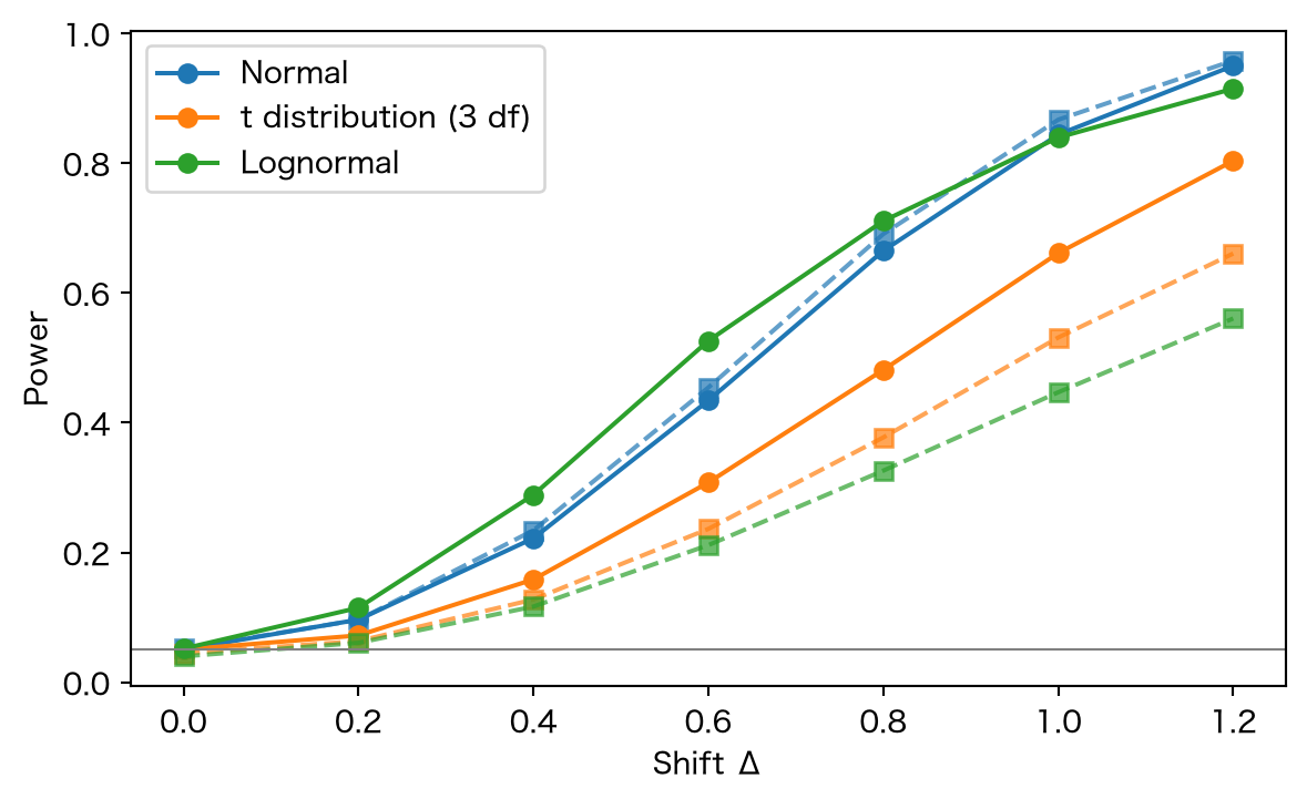
Under normality the t-test is optimal (article on the t-test (Japanese)), but the power lost by rank tests is small. The asymptotic relative efficiency under a pure location shift (the reciprocal of the ratio of sample sizes needed for equal power) is \(3/\pi\approx0.955\) for the normal distribution, at least \(0.864\) for every distribution, and can be much larger than 1 for heavy-tailed distributions (Hodges and Lehmann 1956).
Code
import numpy as npimport matplotlib.pyplot as pltfrom scipy import statsplt.rcParams["font.family"] = ["Hiragino Sans", "sans-serif"]rng = np.random.default_rng(0)n, reps =20, 10000deltas = np.linspace(0, 1.2, 7)dists = {"Normal": lambda s: rng.normal(size=s),"t distribution (3 df)": lambda s: rng.standard_t(3, size=s),"Lognormal": lambda s: rng.lognormal(0, 1, size=s),}fig, ax = plt.subplots()for name, gen in dists.items(): mw, tt = [], []for d in deltas: x, y = gen((reps, n)) + d, gen((reps, n)) mw.append((stats.mannwhitneyu(x, y, axis=1, method="asymptotic").pvalue <0.05).mean()) tt.append((stats.ttest_ind(x, y, axis=1).pvalue <0.05).mean()) line, = ax.plot(deltas, mw, "o-", label=name) ax.plot(deltas, tt, "s--", color=line.get_color(), alpha=0.7)ax.axhline(0.05, color="gray", lw=0.8)ax.set_xlabel("Shift Δ")ax.set_ylabel("Power")ax.legend()plt.show()
Figure 1: Power for two samples (n = 20 each) when x is shifted by Δ (α = 0.05, 10,000 replications per point). Solid lines: Mann–Whitney; dashed lines: t-test. For the lognormal distribution the shift is per unit of scale.
Under normality the t-test is only slightly better, but for the heavy-tailed t distribution and the skewed lognormal distribution Mann–Whitney is far better (about 0.71 versus 0.33 for the lognormal at \(\Delta=0.8\)). However extreme an outlier is, as a rank it is merely the maximum, whereas the standard deviation in the t-test is greatly inflated by outliers.
When the variances differ
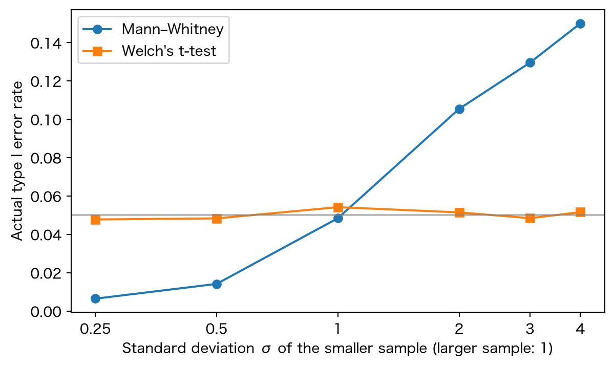
The null hypothesis of Mann–Whitney is \(F=G\), not merely equal medians or \(\theta=\frac12\). If the centers are equal but the variances differ, the variance of \(U_1\) differs from the value in Theorem 2, and the significance level is not maintained.
Code
m, n2, reps =10, 40, 20000sigmas = [0.25, 0.5, 1, 2, 3, 4]mw_rate, welch_rate = [], []for s in sigmas: x, y = rng.normal(0, s, (reps, m)), rng.normal(0, 1, (reps, n2)) mw_rate.append((stats.mannwhitneyu(x, y, axis=1, method="asymptotic").pvalue <0.05).mean()) welch_rate.append((stats.ttest_ind(x, y, axis=1, equal_var=False).pvalue <0.05).mean())fig, ax = plt.subplots()ax.plot(sigmas, mw_rate, "o-", label="Mann–Whitney")ax.plot(sigmas, welch_rate, "s-", label="Welch's t-test")ax.axhline(0.05, color="gray", lw=0.8)ax.set_xscale("log", base=2)ax.set_xticks(sigmas, [str(s) for s in sigmas])ax.set_xlabel("Standard deviation σ of the smaller sample (larger sample: 1)")ax.set_ylabel("Actual type I error rate")ax.legend()plt.show()
Figure 2: Actual type I error rate at the 5% significance level for two samples with the same center (both symmetric about 0) but different variances (20,000 replications each). m = 10 (standard deviation σ), n = 40 (standard deviation 1).
When the smaller sample has the larger variance, the error rate far exceeds 5% (about 13% at \(\sigma=3\)); in the opposite case the test becomes extremely conservative. This is the same structural problem as the equal-variance assumption of the t-test, and converting to ranks does not remove it. If you want to study “the difference in medians” while the variances also differ, consider Welch’s t-test, the Brunner–Munzel test, or a bootstrap confidence interval for the Hodges–Lehmann estimator.
Try it
The same computations are available from the noisymoon API at POST /v1/tests/mannwhitney, wilcoxon and kruskal. The statistics and p-values agree with scipy’s mannwhitneyu / wilcoxon / kruskal.
Lehmann, E. L. (2006). Nonparametrics: Statistical Methods Based on Ranks, revised ed. Springer. Chapters 1–5.
Mann, H. B. and Whitney, D. R. (1947). On a test of whether one of two random variables is stochastically larger than the other. Annals of Mathematical Statistics, 18, 50–60.
Wilcoxon, F. (1945). Individual comparisons by ranking methods. Biometrics Bulletin, 1, 80–83.
Kruskal, W. H. and Wallis, W. A. (1952). Use of ranks in one-criterion variance analysis. Journal of the American Statistical Association, 47, 583–621.
Hodges, J. L. and Lehmann, E. L. (1956). The efficiency of some nonparametric competitors of the t-test. Annals of Mathematical Statistics, 27, 324–335.
Pratt, J. W. (1959). Remarks on zeros and ties in the Wilcoxon signed rank procedures. Journal of the American Statistical Association, 54, 655–667.
Cureton, E. E. (1967). The normal approximation to the signed-rank sampling distribution when zero differences are present. Journal of the American Statistical Association, 62, 1068–1069.
Fagerland, M. W. and Sandvik, L. (2009). The Wilcoxon–Mann–Whitney test under scrutiny. Statistics in Medicine, 28, 1487–1497.